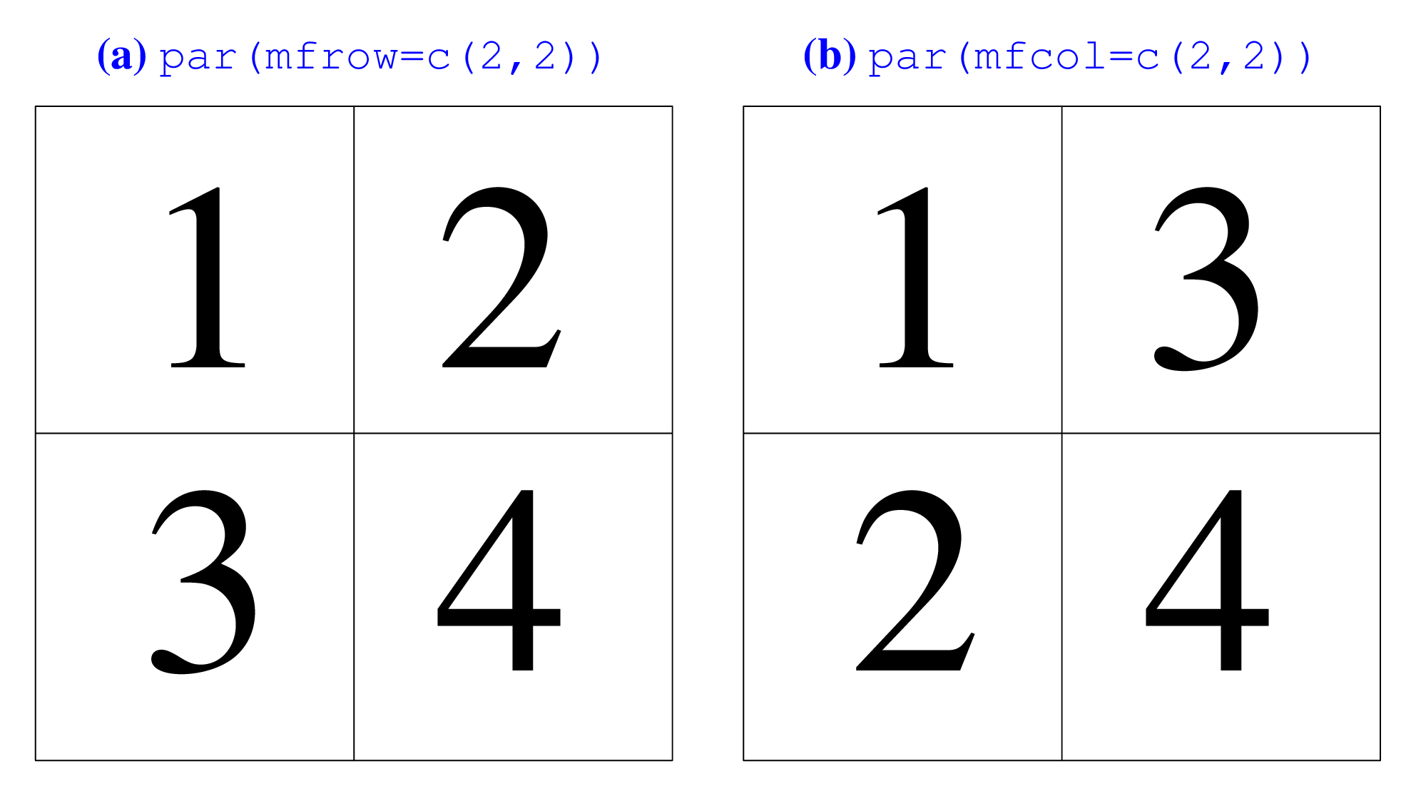
Figure 1: Order of graphs in 2x2 plots set up by (a) mfrow
and (b) mfcol.
Graphs are important tools for making sense of our data and communicating our results. R provides many graphical routines to produce graphs that visualize data in useful ways. We have already worked with a few basic graphs in R. In this section, we will work with graphics in some detail.
As usual, first we will introduce some new data to work with. The new data set comes from a corpus study of child language acquisition. In a nutshell, the study is about how children may be extracting words out of a continuous data stream. Particularly, we are interested whether a set of statistics is helpful for identifying the word boundaries. The data can be found at http://coltekin.net/cagri/R/data/seg.csv. It contains four different statistics: (pointwise mutual information (PMI), successor variety (SV), boundary entropy (H) and reverse boundary entropy (RH) ) calculated on all potential boundary locations for three child-directed utterances. The details are not that important for our purposes here, but if you like to know more about it, the data comes from Çöltekin [2011].
Make sure that all columns in the data frame has sensible data types. Do appropriate conversions if necessary.
We used the plot() function before for scatter plots. This function behaves differently depending of the type of object to be plotted. In the simplest case, you can give a simple list of numbers, and plot() will plot them against their index, i.e., integers starting with one up to the number of elements in the data provided.
Plot the linear regression line over the scatter plot in blue.
If you plot a data frame with plot(), it will result in a matrix of scatter plots where each variable is plotted against the other.
TIP: remember that you can extract the relevant columns of the data frame with the syntax seg[,4:7], or using symbolic names like seg[,c(’pmi’, ’h’, ’rh’, ’sv’)].
We will see more examples of plotting different types of objects, and prettifying the plots like the one in the exercises above. For now, we will first exercise with some of the basic graphics we have seen before, and build on them slowly towards more advanced and nice-looking graphs.
So far, we have used plot() for plotting relations between two samples. We can also plot mathematical functions. For example, the following plots the well-known bell curve of the Gaussian function.
> x <- seq(-4,4,by=0.1)
> plot(x, dnorm(x))
We first create a vector variable that holds numbers between to , and plot these number against dnorm(), which returns the value of the normal density function (more on density functions later). If you run the above command, you will see a set of dots tracing the standard Gaussian curve. If you want to see lines connecting these points instead, you can pass the option type=’l’ to the plot() function. Similarly, the option type=’b’ plots both (lines and points).
It would be interesting to see both the normal and t distributions on the same graph. However, every time we run a plot() command R clears the earlier plot, and initializes a new ‘canvas’. We have already seen the abline() function which allowed us to plot on an existing plot. There are more functions that draw over an existing graph. Most commonly used ones include,
The colors are useful for distinguishing different lines in a graph. However, the color distinction will be unreliable in black-and-white print. A common practice for identifying different lines on the same graph is to use different line types, or patterns. The commands that draw lines allow you to specify a different pattern using the option lty. For example, setting lty=2 in plot() or lines() will draw a dashed line (the default is 1, which draws a ’solid’ line). Alternatively, you can use symbolic names like ’dotted’, ’dashed’ etc.
Similar to lty that sets the line-pattern, you can also customize the type of the points drawn by plot() or points(). The parameter that decides the shape of the points drawn is pch. If you provide a single-character text string to pch it will use this character instead of the default. Alternatively, you can provide a numeric value to obtain a number of predefined shapes. For example pch=22 will plot a filled square (see help text for points() for other symbols).
With the text() command, you can place an arbitrary text on any point in the x-y plane. In its typical use, it is used like text(x, y, labels), where all arguments are vectors of equal size. Furthermore, you can adjust the position of the labels with pos and offset options (see help text for more information).
** Use red for the phonemes that correspond to boundaries and blue for word-internal locations.
This exercise, especially the last part, is rather tricky, but you have all the tools at hand to achieve this.
In graphs like the ones in exercises 6.9 and 6.10, we typically include a legend to explain what colors or patterns mean. The command legend() in R adds a legend to an existing plot.
We improved the graph in Exercise 6.14 quite a bit, it is almost ready to be printed. However, the y-axis is labeled as ‘dnorm(x)’ which definitely is not the typical axis label found in printed material. You can specify the axis labels using xlab and ylab options, and a title on top with the option main.
By default R determines for a reasonable x-y region for your plots when you use plot() and the other functions that initialize a new graph. Sometimes, you may want to change the range of the values on the x- or the y-axis. Often you need to do this to make sure that the subsequent points() and lines() fit into the canvas prepared by a plotting function, sometimes you may want to extend one of the axes to leave some space for your legend, and sometimes you may want to include a particular reference point, for example, the origin (coordinates ) in the graph no matter what data to be plotted. To set the ranges that will be visible on a graph we use xlim and ylim parameters to the plotting functions. For example, xlim=c(0, 10) will result in the x-axis to cover the range between and . Note that any graphics drawn outside the region specified by xlim and ylim will be clipped out, they will not be visible.
Often, we would like to display more than one graph on the same figure in a publication or presentation. One way to achieve this is to set one of the graphical parameters mfrow or mfcol. The graphical parameters in R are set using the command par(). Once set, these parameters will be effective for all graphics related commands. For mfrow and mfcol we specify a two-element vector, where the first element specify the number of rows, and the second one specifies the number of columns. For example, the command par(mfrow=c(4,5)) creates a grid of four rows and five columns where next 20 plot() (or others like hist(), boxplot()) commands will place their output. The difference between mfrow and mfcol is the order of the plots. mfrow fills the specified grid following a row order, while mfcol fills the columns first. Figure 1 shows the order of graphs produced with mfrow and mfcol options.
Plot four graphs on a 2x2 grid on the same canvas each displaying side-by-side box plots for boundary and non-boundary positions for pmi, h, rh and sv values. Set the main title accordingly to identify the graphs.
The par() command sets many other graphical parameters. Some of these parameters, e.g., pch or lwd, serve as defaults to the later graphical commands, and can be overridden by the later commands like plot(). Some others, like mfrow, affect behavior that you cannot set through the individual commands. You are encouraged to skim through the help text for par() to get an impression of the parts of the R graphics that you can customize.
Once you are happy with your graph, you will want to include it in your presentations and/or publications. You can, of course, get a screenshot, but in most cases, this method produces less than optimal graphics, especially for publishing. R supports a number of formats that produces ‘publication quality’ graphs. The possible file formats include Postscript, PDF, PNG and JPEG. Typically, if you want to have a bitmap file (for the web and possibly for your presentations), you should use PNG graphics. If it is for a publication, you should pick a vector file format, such as PDF (If you are a LATEX user, you should definitely check tikzDevice, though).
To plot your graphics to an external file, you first need to use appropriate function to initialize the output ‘device’. The initialization functions are typically the (lowercase) name of the graphics format you are interested in. For example, pdf(), postscript(), png() or tiff(). These functions somewhat differ depending on the file type you want to produce, but in almost all cases you need to specify a filename and the width and height of the resulting graphics. For bitmap graphics, the width and height are specified in pixels, for vector graphics it is specified in physical dimensions, e.g., in inches. You should consult the documentation of the functions you want to use. In general it is important to specify the correct size since some properties of the resulting graph, such as font sizes and line thickness, will be determined based on the size of the graphics. Once you have initialized the output, the commands you use for producing graphs are the same. When you are done with plotting your graph(s), you should type dev.off(). The resulting graphics will be written to the file you specified during the initialization.
Using abline(), add horizontal and vertical lines that pass from the origin (0,0) to the graph you produced in Exercise 6.24.